Analyzing Complex Network metrics from the 1958 World Cup final
The World Cup is the most important football competition in the world. It is held every four years and gathers the best national teams in the world. The first edition of the competition was held in 1930, in Uruguay, and since then, the competition has been held every four years, except in 1942 and 1946, due to World War II. The competition is organized by FIFA (Fédération Internationale de Football Association), the world's football governing body.
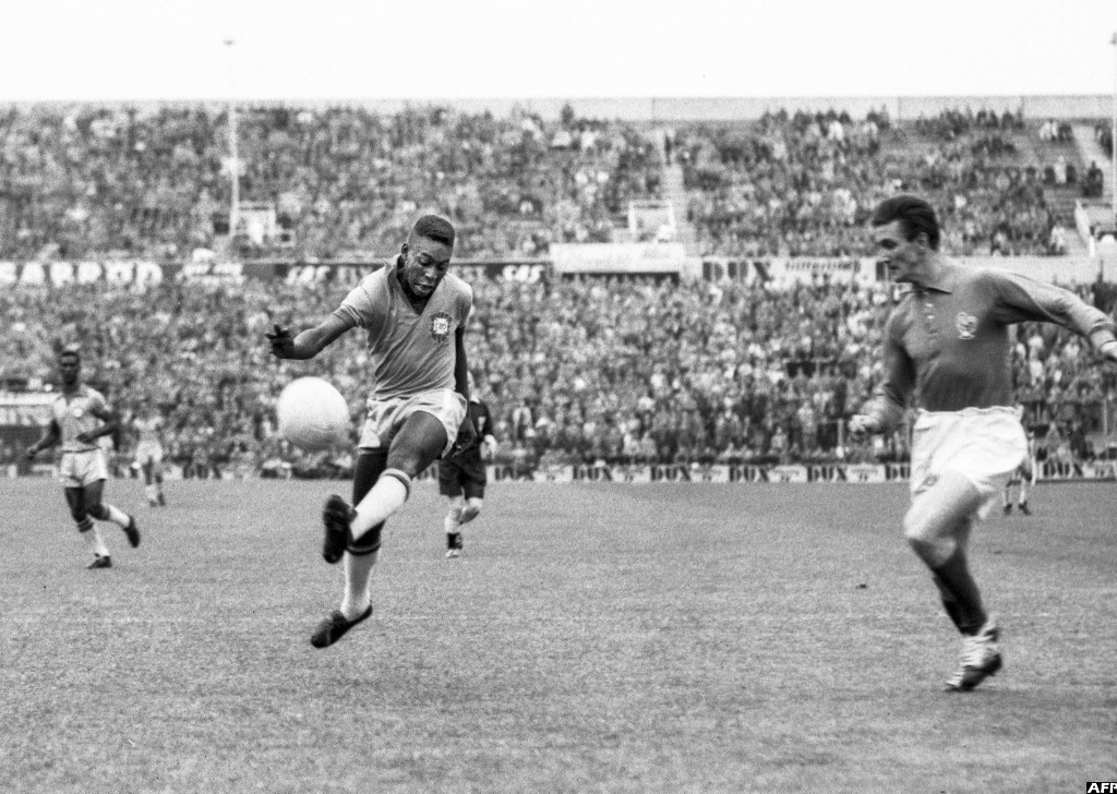
The 1958 World Cup was the sixth edition of the competition and was held in Sweden. The competition was attended by 16 teams, which were divided into four groups of four teams each. The first two teams in each group advanced to the quarterfinals. The competition was won by Brazil, which beat Sweden 5-2 in the final. The Brazilian team was led by the legendary Pelé, who was only 17 years old at the time.
This post aims to analyze the 1958 World Cup final passes networks between the Brazilian players. The data used in this post was obtained from the StatsBomb Open Data repository. We will explore some Complex Network metrics to investigate the Brazilian team's passing network in the final match. Let's code!
Data extraction
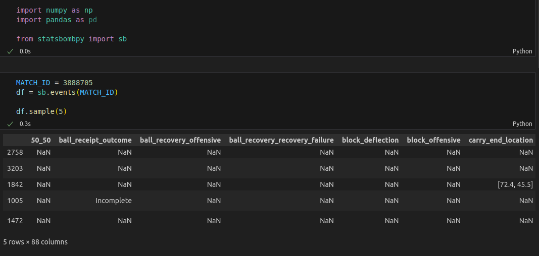
The data extraction process can be considered the easiest one. It is because Statsbomb provides a Python package called statsbombpy that allows us to extract the data directly from the repository based on the match_id that they provide in the repository. The extraction would be as follows:
Data preparation (to the passes network)
With the DataFrame from avents loaded, we can begin creating a class for the players and a function to get all the Starting XI players from the match (the ones that we will use in the passes network). The class for the players is as follows:
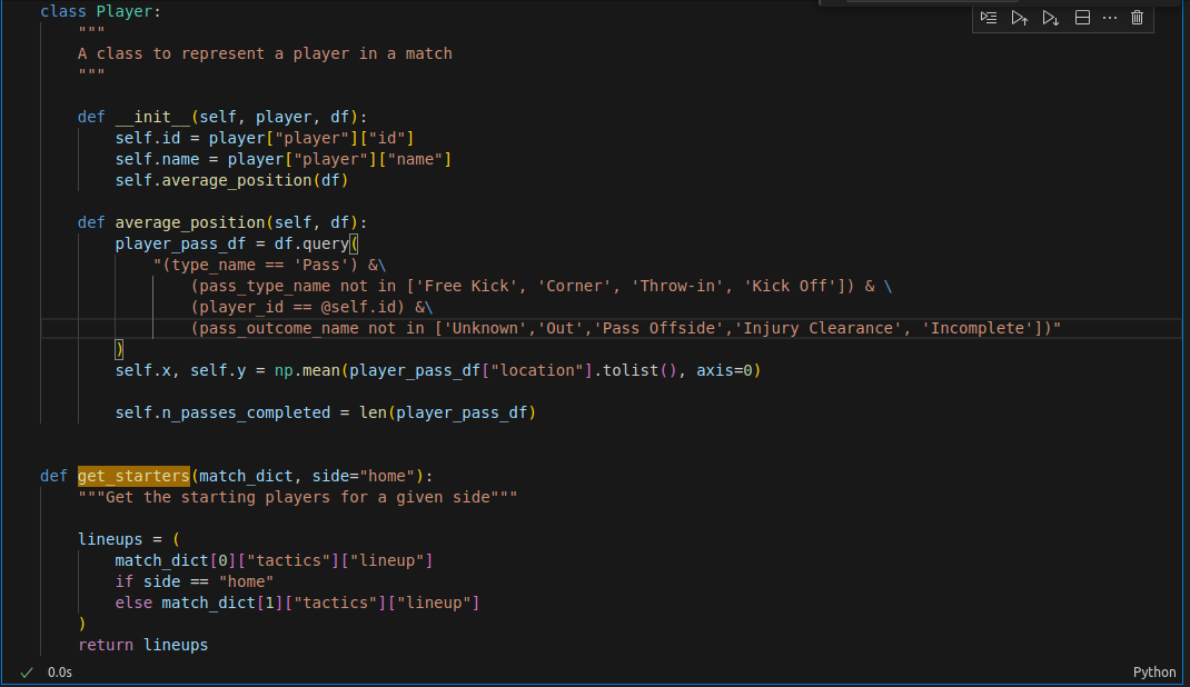
Using our DataFrame we want to filter the data following some criteria, so:
- The event must be a pass
- It cannot be a pass from set-pieces
- And it must have an outcome of success
After this filtering, we aggregate the data by the player that made the pass and the player that received the pass. And that's it, we have our passes network.
Analysis
Now that we have our passes network, we can start the analysis. The first thing we can do is to plot the network. We can do this using the NetworkX package. The result will be like this:
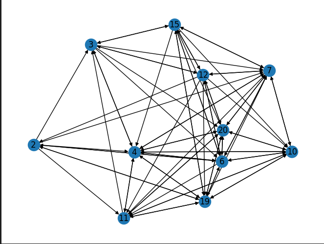
Yeah... It's not very informative. We can see that Pelé is the player who receives the most passes, but we can't extract much information from this plot. So, let's try to improve it...
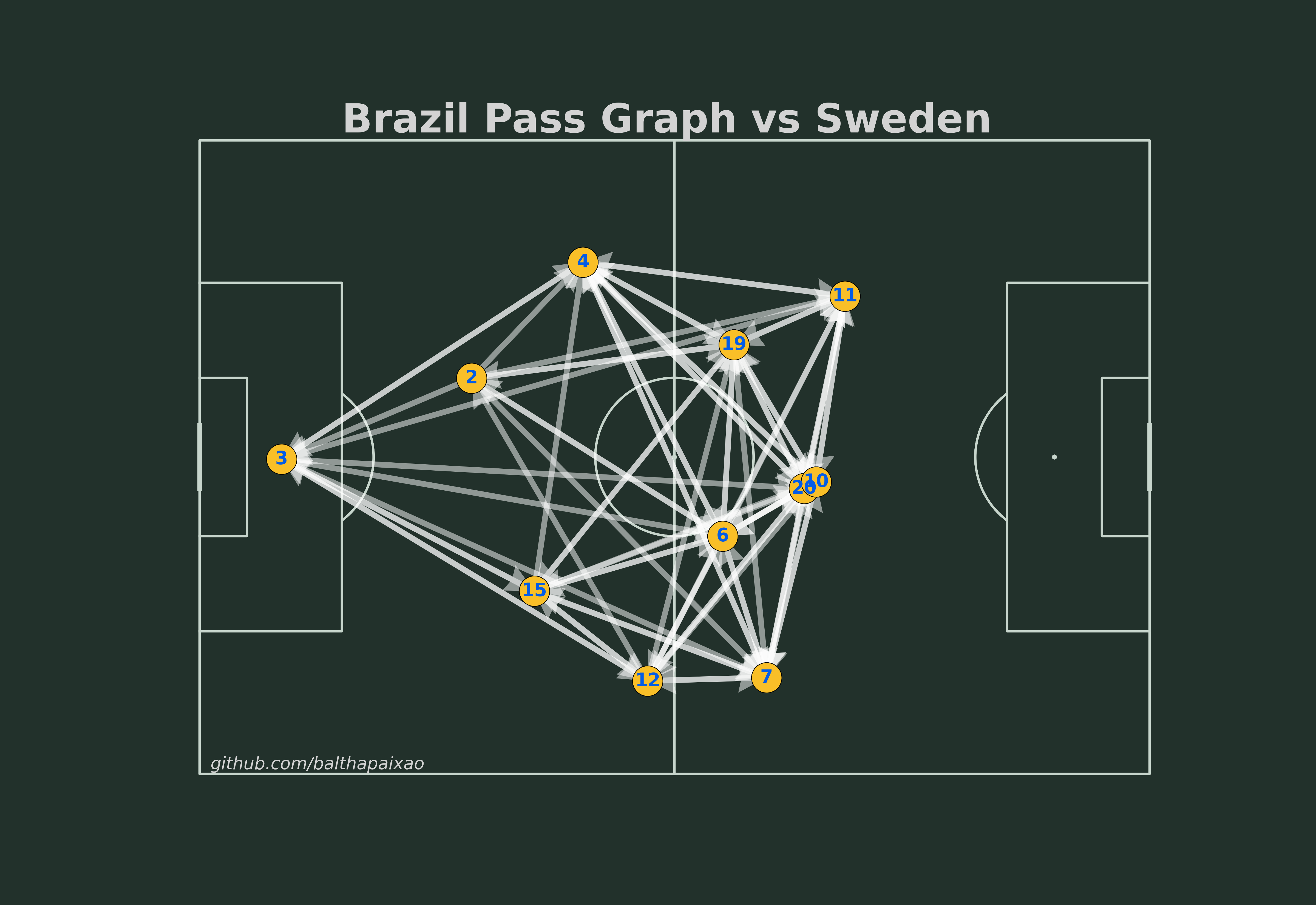
Much better! Now we can see that Pelé and Vavá are occupying almost the same average position in the field. We can also see some differences compared with modern football. For example, there is no player with an average position in the center of the field.
Complex Network metrics
As could be noted, we explore the creation of a pass network where our graph is a DiGraph, i.e., a directed graph. This is because we are interested in the direction of the passes. Given that, we can explore some Complex Network metrics to investigate the Brazilian team's passing network in the final match and their behavior.
Degrees
The degree of a node is the number of edges incident to the node, the passes between the players. The player that showed the lowest degree was, unexpectedly, Bellini; and the player that showed the highest degree was Waldir. This could indicate how Brazil was exploiting spaces on the right side of the field. The average degree was 14.2. One interesting thing is that Pelé is not the player that received the most passes, the player is Garrincha.
Clustering Coefficient
Clustering indicates how close a node and its neighbors are to being a clique. In our case, it indicates how close a player and his teammates are to being a clique (a group of players that pass the ball between them). The player that showed the highest clustering coefficient was Pelé. This could indicate that Pelé was the player that was more involved in the passing game. The lowest clustering coefficient was shown by Gylmar, the goalkeeper, which is expected.
Closeness Centrality
Closeness centrality indicates how close a node is to all other nodes in the network. In our case, it indicates how close a player is to all other players in the network. The player that showed the highest closeness centrality was Garrincha, one of the most important players regarding dribbling and creating chances. The lowest closeness centrality was shown by Bellini, as the game was not being explored on his side of the field based on our theory.
Betweenness Centrality
Betweenness centrality indicates how often a node appears on a shortest path between two other nodes. In our case, it indicates how often a player appears on a shortest path between two other players. The player that showed the highest betweenness centrality was Waldir, while the lowest betweenness centrality was shown by Bellini, which indicates that our beliefs are correct.
Hubs and Authorities
Hubs and Authorities are two metrics that are used to identify how the degrees are distributed between the nodes in a network. The Hubs metric identifies the nodes that passed the ball the most, while the Authorities metric identifies the nodes that received the ball the most. The player that showed the highest Hubs metric was Waldir, and the player that showed the highest Authorities metric was Pelé. This indicates that Waldir was the player who passed the ball the most, while Pelé was the player who received the ball the most.
Pagerank
Pagerank is a metric that is used to identify the nodes that are more important in a network. The player that showed the highest Pagerank was Pelé, and the player that showed the lowest Pagerank was Bellini. This indicates that Pelé was the player that was more important in the network, while Bellini was the player that was less important in the network.
Conclusion
In this post, we analyzed the 1958 World Cup final passes network between the Brazilian players. We explored some Complex Network metrics to investigate the Brazilian team's passing network in the final match and their behavior. We found that Pelé, Garrincha and Waldir showed a great importance in the network, while Bellini and Gylmar showed a low importance in the network. We also found that Brazil was exploiting spaces on the right side of the field.
I hope you enjoyed this post and could learn a little bit more about complex networks. If you have any questions or suggestions, please leave a comment below. The complete analysis code can be found on the notebook.
Enjoy Reading This Article?
Here are some more articles you might like to read next: