In this post, we will present another method for predicting victory. This time, we will use the market value of the teams as the main variable, which corresponds to the sum of the individual market values of all players on the team. We will explore how this metric can influence the performance of clubs and their chances of winning a match.
Context
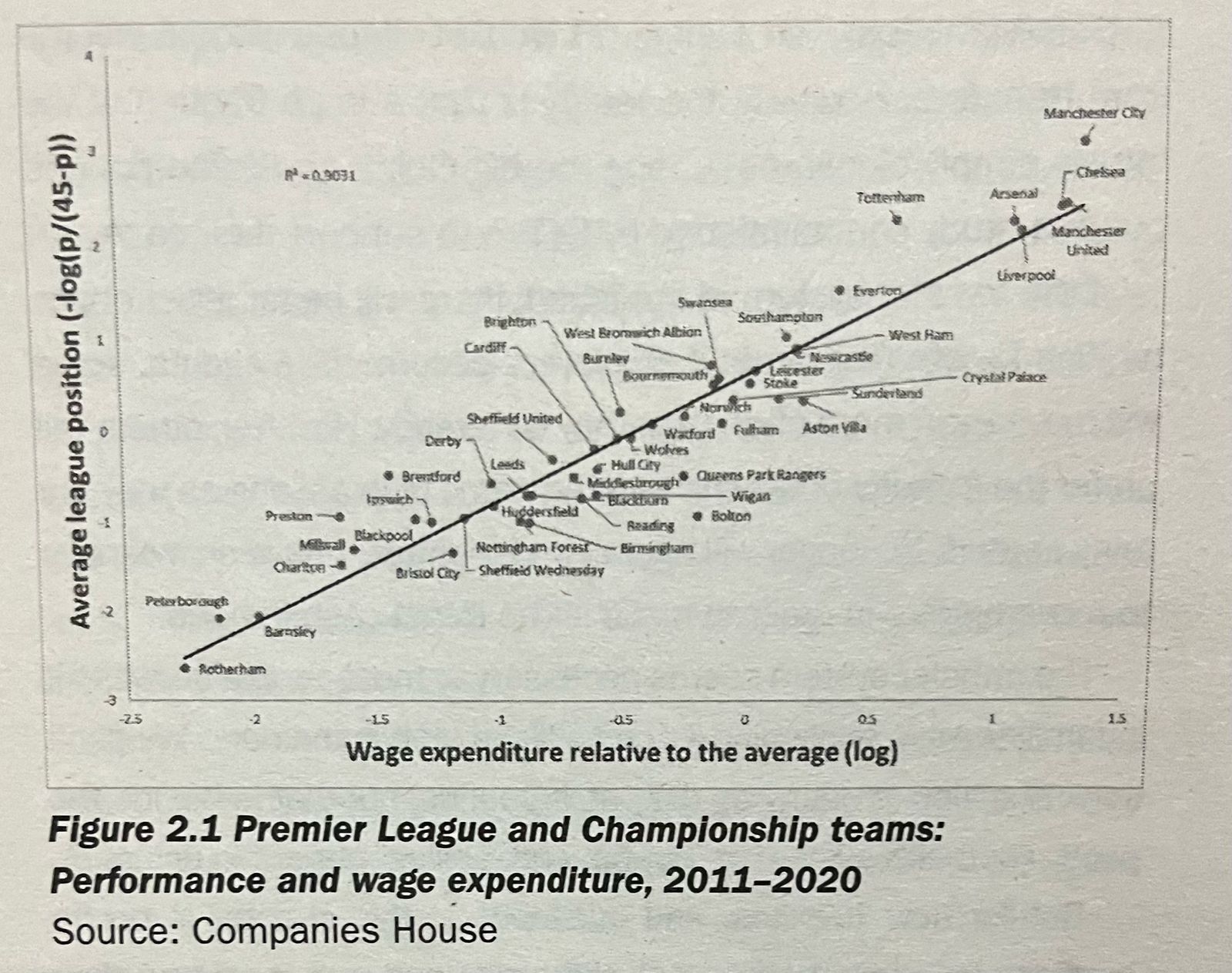
Money plays a significant role in modern football. With the transfer market becoming increasingly inflated, it is necessary to spend more money in the transfer windows to maintain competitiveness in the top leagues. The professionalization of the sport has also had a great influence on increasing the cost of maintaining a team, as more expenses are now needed for infrastructure and creating a quality environment to stay ahead of the competition. In fact, studies in the Premier League and Championship (2011-2020) have shown a correlation between a team's payroll and the position the team achieves in the table (Soccernomics, Simon Kuper and Stefan Szymanski). Money drives football. Therefore, we will use the market value of the clubs in the Brazilian league to try to predict the final result of the matches.
Method
Data
We will use data from the 2023 season. The dataset has two main parts:
The match data: information such as the home team, away team, result, match date, and odds for victory (home, draw, away), extracted from the Football-data website and the Pinnacle betting house.
The market value of the teams in the Brazilian league 2023, sourced from Transfermarkt.
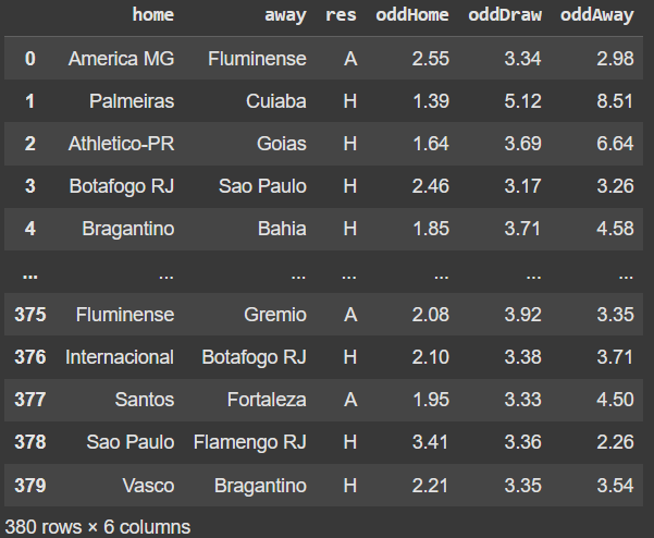
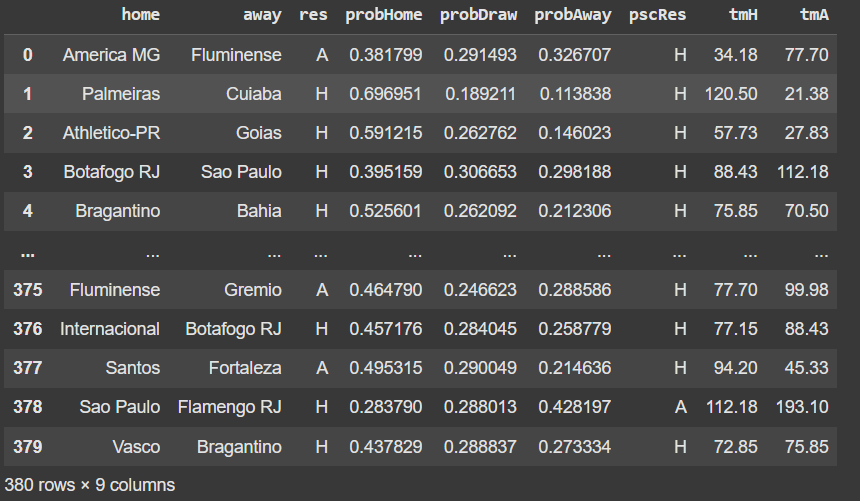
Let’s take a look at our match dataset. It has about 19 fields, but only the following are relevant to us:
Legend: home: Home team; away: Away team; res: Match result; oddHome: Home team's chance of victory; oddDraw: Chance of a draw; oddAway: Away team's chance of victory.
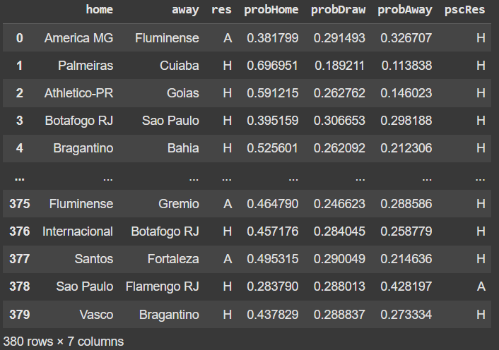
We will transform the odds into probabilities. To do this, we don't simply use the formula (1/odds), because the sum of the probabilities would exceed 1. This excess represents the bookmaker's margin, so we normalize the probabilities to correct it.
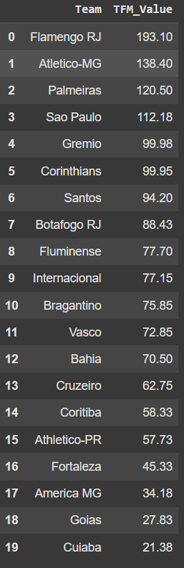
Now let's take a look at the market value data:
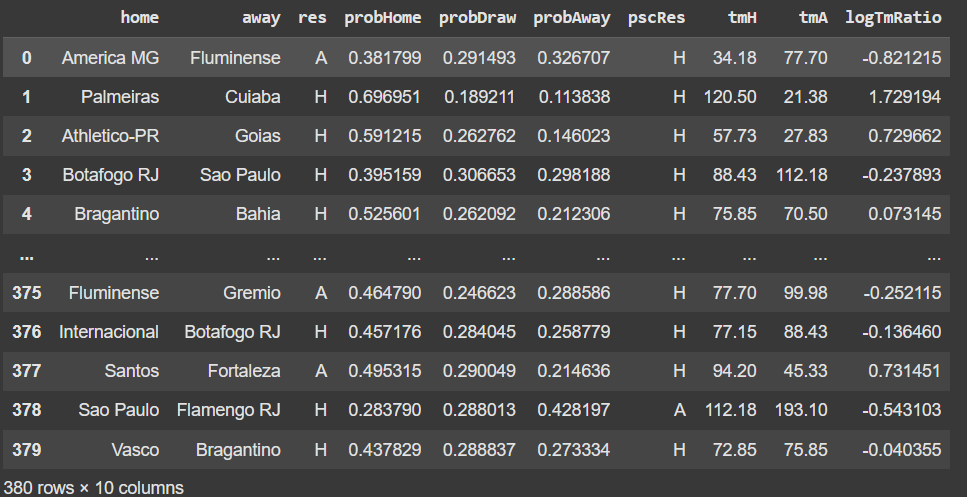
The column TFM_Value contains the market value in millions of euros. For example, Palmeiras' market value is 138.4 million euros. These values represent the market values of the clubs as of July 20, 2024. We have merged the two datasets, adding the market value columns for the home team (tmH) and the away team (tmA).
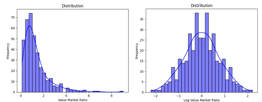
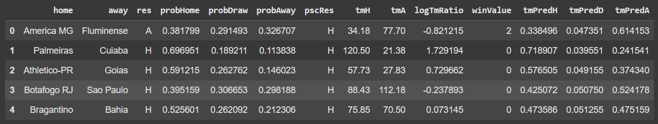
The variable we will use to predict the results is the ratio between tmH (home team's market value) and tmA (away team's market value). More specifically, the logarithm of this ratio. The reason we use the log is that the distribution of the ratio between tmH and tmA is skewed to the right. Applying the log function makes the distribution symmetrical, which improves performance. The image below helps to visualize this.
So, the logTmRatio will be the variable we will use to predict the results. In other words, our independent variable.
We encoded the res column as:
0: Home team victory
1: Draw
2: Away team victory
This new column will be called winValue.
Model
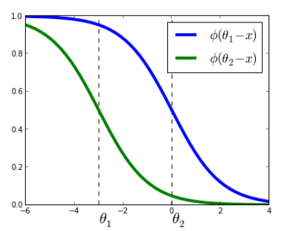
We will use an Ordinal Logistic Regression model, which is a technique used to model the relationship between an ordinal response variable (i.e., categories with order) and one or more predictor variables. In our case, the ordinal response variable is winValue and the predictor variable will be logTmRatio. The model involves determining the \( \alpha_1 \), which is the point that separates the home team victory from the draw or away team victory. In other words, if a point falls before \( \alpha_1 \), the model will predict a home team victory, and if it falls after \( \alpha_1 \), it will predict a draw or away team victory. The \( \alpha_2 \) is the point that separates the draw from the away team victory. The \( \beta \) indicates how the predictor variable, in our case the market value ratio, influences the result. For better visualization of this explanation, observe the graph below, where \( \alpha_1 \) is represented by \( \theta_1 \):
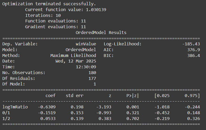
We used an Ordinal Logistic Regression model, which relates an ordinal response variable (winValue) to a continuous predictor (logTmRatio). The model finds two cutoff points:
\( \alpha_1 \): separates home team victory from draw or away team victory
\( \alpha_2 \): separates draw from away team victory
\( \beta \): tells us how this ratio influences the result of The coefficient of logTmRatio
Now that we understand the model, let's prepare its training. The training dataset consists of the first 200 games of the season, and the remaining 180 games will be used as the test dataset.
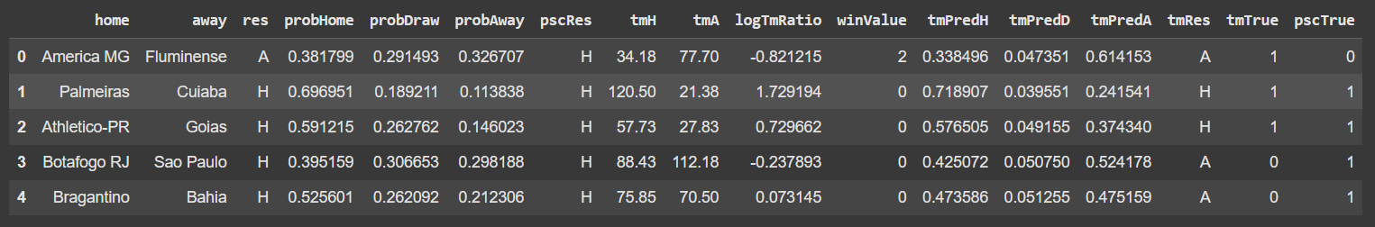
Let's add columns to compare the prediction results from Pinnacle and what we found.
Evaluation
Remember that we used the first 200 games to train our model, so we will compare the prediction results from our test set.
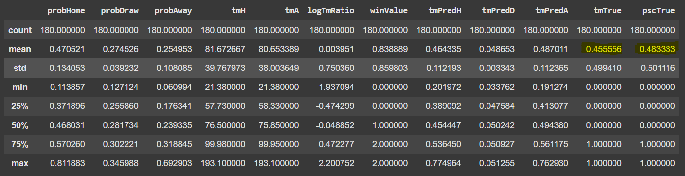
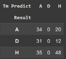
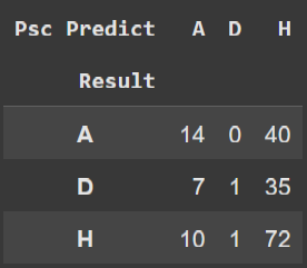
The most important value for us is highlighted: the average accuracy of results from both the bookmaker and our model. Notice that they are close, and even the bookmaker had less than 50% accuracy. One important thing to consider when analyzing these data is the size of the training set, which only had 200 matches, and we achieved a result of a 0.03 difference from the bookmaker. Let’s create two cross tables to better understand in which types of games our model is most likely to make errors and succeed.
Notice that in the draw column, our model did not predict draws, which is due to the fact that the market value ratio between two teams has a very low probability of resulting in a draw, since it is expected that the market values of the teams would need to be close to each other.
The numbers are quite scattered, but we can see that our model performs better than Pinnacle in predicting away team victories, while Pinnacle has most of its correct predictions in home team victories.
Conclusion
In the next post, we will discuss the prediction of results based on the Poisson distribution, a well-known distribution used to predict rare events. Stay tuned to our social media to not miss any updates from the blog!
Enjoy Reading This Article?
Here are some more articles you might like to read next: