Comparing the Performance of Predictive Models – 2026 World Cup
Se quiser ler esse texto em pt-br, clique aqui.
Introduction
Before the start of a World Cup, several research groups, media outlets, and technology companies publish predictions about how national teams will perform in the competition. It is only after the tournament ends, however, that it becomes possible to check those predictions against what actually happened on the field. That is exactly what we do in this post: we evaluate the performance of the predictive models developed by the ACE Laboratory for the 2026 World Cup, comparing them against one another and against other public benchmarks.
This comparison is especially relevant for a tournament like this edition — the first to feature 48 national teams — which was marked by surprises in both directions: lower-profile teams such as Cape Verde and Egypt put up serious resistance before being eliminated, while traditional favorites like Germany and the Netherlands fell as early as the round of 32, and Brazil did not make it past the round of 16. Throughout this post, we show how to compare the performance of different predictive models in this unpredictable scenario — and what these results reveal about the laboratory’s models.
The Laboratory's Models
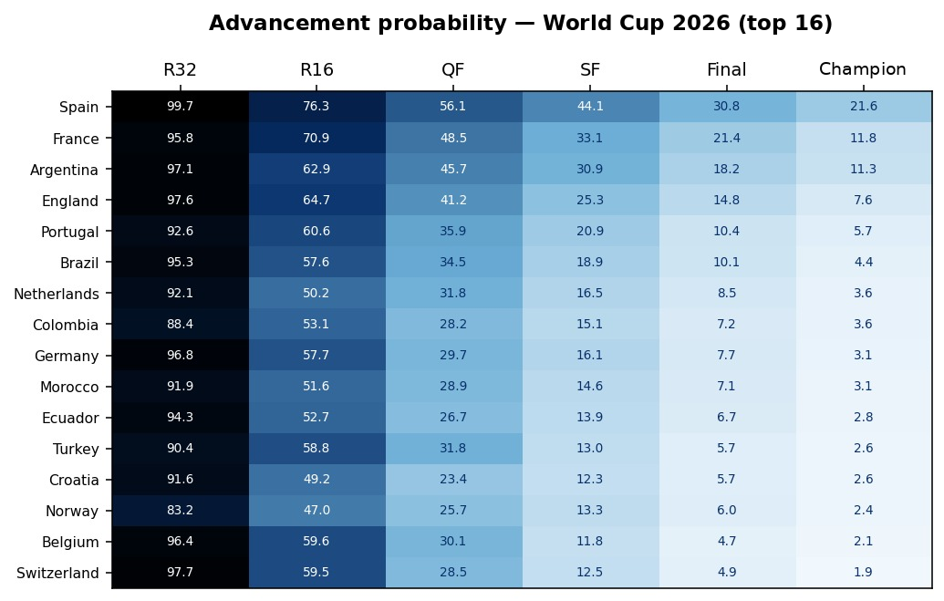
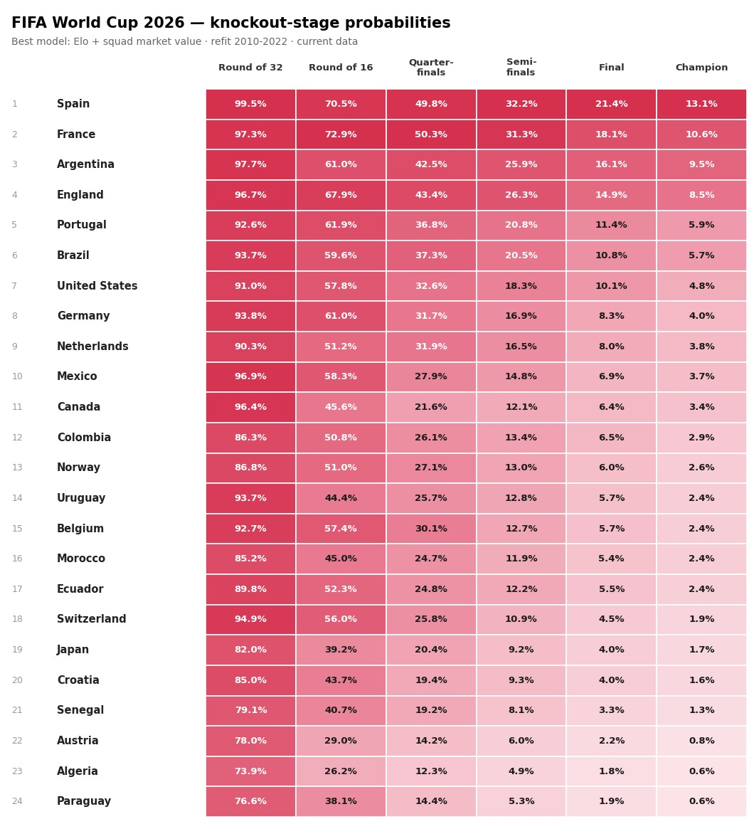
In addition to the Ensemble model, which was used as the basis for the World Cup predictions, the ACE Laboratory developed two other models. All of them use the structure of the Dixon-Coles Model, but each one estimates the distribution’s parameters differently. In all cases, the input data was based on recent results and the historical strength of each national team. The Ensemble model, as explained in the first post, assigns equal weight to three different methodologies; the Bayesian model uses the data to define a prior distribution; and the Classic model estimates the parameters directly. In the images below, we show the advancement probabilities generated by the Bayesian and Classic models for each stage.
Comparing with other models
Now that the World Cup is over and we have all the results, we can finally measure the performance of the models created by the laboratory. To make this analysis even more complete, we will compare our models’ predictions with three other predictions generated by different models that are relevant in the world of football data analysis: Gato Mestre (Globo), Opta — which only released probabilities starting from the quarterfinals — and UFMG.
Overall, the models analyzed performed well in pointing to Spain as champion, with the exception of the UFMG model, which assigned only a 3.0% probability to the Spanish team, versus 5.9% for Argentina. This result, on its own, is not enough to assess the quality of a model: it is possible to get the champion right and still make significant errors in the rest of the predictions. There is also the risk that models which spread probabilities close to the average are not penalized for doing so, making them not very useful for decision-making. What is needed, then, is an evaluation criterion capable of rewarding correct calls made with confidence and penalizing mistakes made with that same confidence, without letting uninformative models go unnoticed. This type of criterion is known as a proper scoring rule, and that is exactly what the metrics below aim to measure.
Brier Score
\[\frac{1}{N}\sum (p - y)^2\]The Brier Score is the mean squared error of the probability. For the event “the team reached at least stage k,” the probability p assigned by the model and the actual outcome y (1 if the team reached that stage, 0 otherwise) are taken, (p − y)² is calculated, and the arithmetic mean is taken across all cells — that is, every combination of team and stage. The lower the value, the better the model’s performance.
Ranked Probability Score (RPS)
This is our main metric. While the Brier Score treats each stage as an independent event, the RPS takes into account that the stages follow a natural order — group stage, round of 32, round of 16, quarterfinals, semifinals, final, and champion. This metric compares the predicted cumulative probability curve with the observed curve and measures the squared distance between the two, penalizing more severely errors that are further apart in the order: predicting a team as champion and seeing it eliminated in the first stage weighs more heavily than being off by just one stage. The average is calculated across teams, and again, the lower the value, the better.
The two metrics are directly related: for each team, the RPS corresponds exactly to the average Brier Score for that team across the stages. Thus, a model’s RPS is, in practice, the average of its Brier Score across all stages.
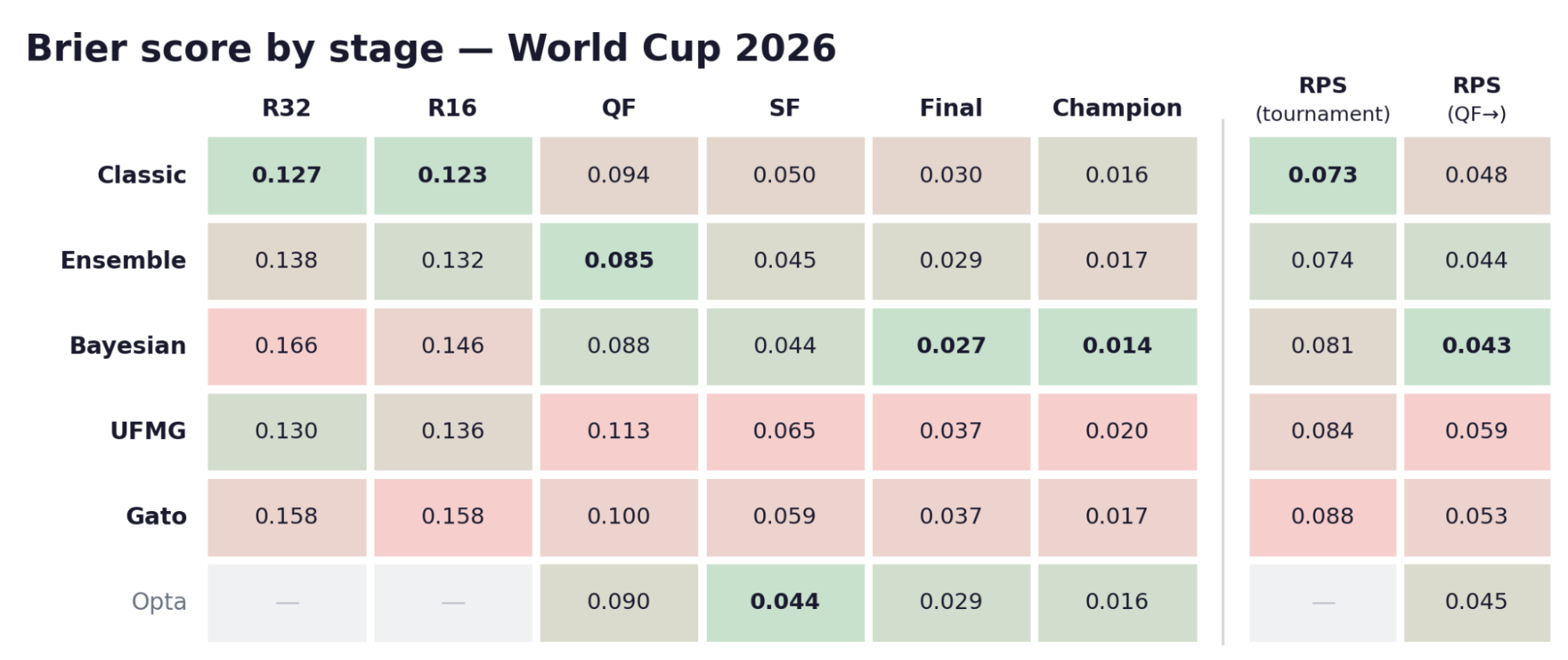
Figure 3 makes the pattern clear. In the early stages (round of 32 and round of 16), the models that erred the least were the Classic, the Ensemble, and UFMG, which better anticipated which teams would advance past the group stage, while the Bayesian model — more confident in the favorites — paid a high price for the stumbles of Germany and the Netherlands. In the quarterfinals, the Ensemble still leads, but from the semifinals onward the picture reverses: the Bayesian and Opta take the lead and do not give it up again, with the Ensemble close behind in every subsequent stage, while UFMG, which had been doing well, drops off sharply. It is in the decisive stages that well-placed confidence in the favorites pays off, since the competition did not produce many upsets at that point — it is worth remembering that Opta only released probabilities starting from the quarterfinals. Overall, the laboratory’s three models performed very well: the Classic and Ensemble lead the tournament’s cumulative RPS, the Bayesian leads the RPS from the quarterfinals onward, and all three stay ahead of Gato Mestre and on par with Opta, the strongest of the external benchmarks.
The RPS and the Brier Score, on their own, only indicate which model made fewer mistakes — they do not explain why. A single number is not enough to distinguish a genuinely informative model from one that simply plays it safe around the average. To understand that difference, and to identify who was confident and right, who was confident and wrong, and who simply avoided taking a position, complementary metrics are needed.
Log-Loss
\[-\frac{1}{N}\sum \left[ y \ln p + (1-y) \ln(1-p) \right]\]Log-Loss follows the same logic as the Brier Score, but penalizes mistakes made with high confidence much more severely. Here, p is the probability assigned by the model and y is the actual outcome (1 if the event occurred, 0 otherwise). Assigning a 99% probability to an event that does not happen sharply raises the score; an error around 55%, on the other hand, is penalized much more mildly. This is the metric that most rewards sharp, well-calibrated models, and the one that most heavily penalizes overconfidence.
Skill Score
\[1 - \frac{S_{\text{model}}}{S_{\text{baseline}}}\]This is not a new metric, but rather a way of interpreting the others: here, S represents the score (RPS, Brier, or Log-Loss) of the model and of a baseline for comparison — in this post, we use the RPS. The baseline corresponds to a naive guess, that is, the base rate: the average frequency with which a team reaches each stage. The Skill Score comes out to 0 when the model merely ties with that naive guess, and to positive values when it beats it. The metric therefore answers a direct question: “how much better than the obvious is this model?” A Skill Score of 37%, for example, indicates a 37% reduction in error relative to simply following the base rate.
Calibration, Resolution and Sharpness
Beyond Log-Loss and the Skill Score, the Brier Score itself can be broken down into two complementary components: Calibration and Resolution. Calibration measures whether the probabilities assigned by the model are honest — on the occasions when the model assigned a 70% probability to an event, did that event actually occur about 70% of the time? (the lower, the better). Resolution, in turn, measures the model’s ability to differentiate between cases, pushing probabilities away from the average in a way that is consistent with the observed outcomes, rather than keeping predictions close to the midpoint for every case (the higher, the better). It is possible, however, for a model to be well calibrated and still not very useful: it gets the average of occurrences right but does not differentiate between cases. Resolution is what rewards the confidence that actually helped discriminate between outcomes.
The models also differ in how much risk they take when issuing their probabilities — which is what Sharpness measures directly, looking only at the predictions themselves, without considering the outcomes: the more a model concentrates probability rather than spreading it across the alternatives, the lower the Sharpness, and the more decisive the model. On its own, however, Sharpness does not say whether a model is good — the merit lies in being sharp without compromising calibration.
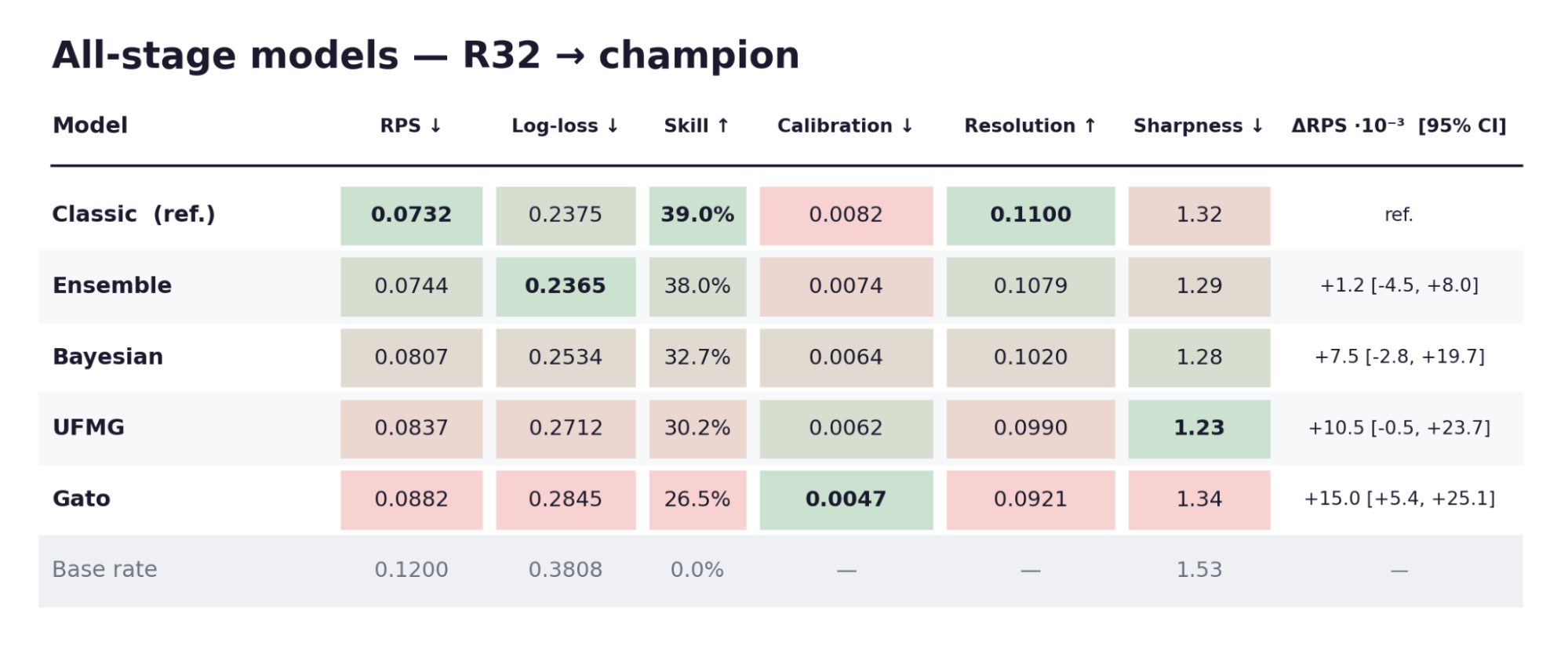
With these complementary metrics in hand, it is possible to revisit the models’ performance across the whole tournament, from the round of 32 to the champion. The Classic model leads the cumulative RPS (0.0732), closely followed by the Ensemble (0.0744) and, at a greater distance, by the Bayesian (0.0807). The ΔRPS column, however, calls for caution in reading these numbers: the confidence intervals for the Ensemble, the Bayesian, and even UFMG cross zero, which indicates that, within a single tournament, it is not possible to statistically separate them from the Classic model with confidence. The only model that clearly lags behind is Gato Mestre, whose confidence interval does not touch zero.
It is also worth noting that the Classic and Ensemble models show the highest Resolution (0.1100 and 0.1079, respectively), having best separated the teams that advanced from those that were eliminated — a result corroborated by Log-Loss, with both models ahead of the others. Gato Mestre, meanwhile, is the best-calibrated model (0.0047), but that isolated advantage did not translate into practical usefulness: as discussed earlier, getting the average probability right is not the same as discriminating well between outcomes.
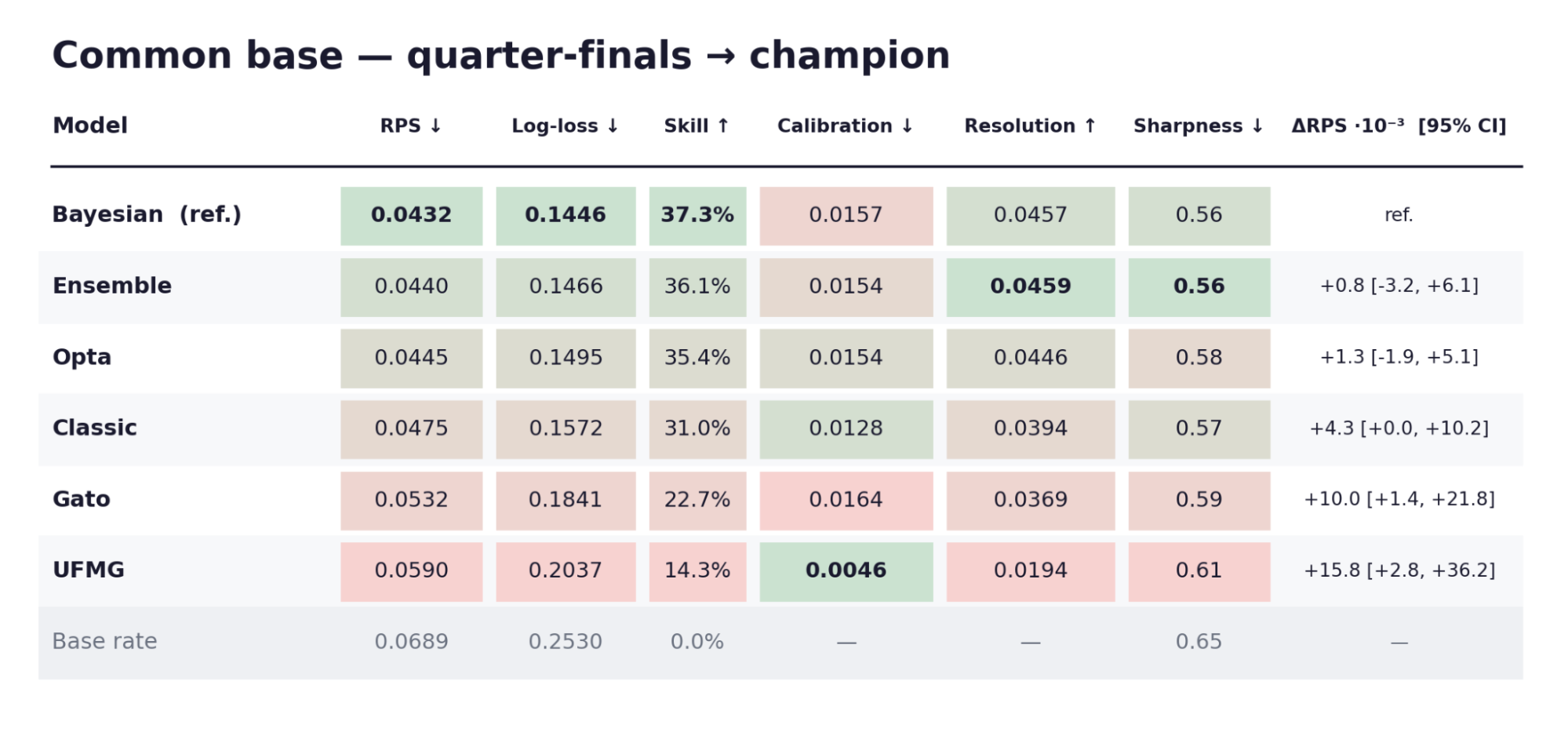
From the quarterfinals onward, the Bayesian model takes the lead (RPS 0.043, best Log-Loss, and best skill, at 37.3%). Even so, the top is a tie: the Ensemble (+0.8) and Opta (+1.3) have intervals that cross zero, meaning the three are statistically indistinguishable. The Bayesian model ends up on par with Opta precisely in the most decisive stages. The Classic model falls back a bit, since its strength lay in the early stages, which are now excluded from this comparison. Gato Mestre and UFMG follow next, now with intervals that do not cross zero. UFMG’s result nicely illustrates the difference between calibration and usefulness: it is the best calibrated (0.0046), but has the lowest resolution (0.019) — honest on average, but not very decisive.
Conclusion
In the end, the most honest reading is that there was no single winner. The lead changes hands depending on the stage: the Classic and Ensemble models make fewer errors in the early rounds, the Bayesian takes over in the decisive ones, and in the stages that determine the champion, all three of the laboratory’s models end up on par with Opta, the most relevant external benchmark. Since this is a single World Cup, many of these differences fall within the margin of uncertainty, which is why we prefer to speak of distinct profiles rather than crown a single champion among the models: each one takes risks in its own way, and each bet pays off at a different moment in the tournament. For the laboratory, this confirms that all three models compete on equal footing with the best public benchmarks, and it also points to a path forward: accumulating more tournament editions to reduce that uncertainty.
⚠️ Disclaimer
This study was developed exclusively for academic and research purposes, with the aim of testing and refining data science models. Football is unpredictable, and the results presented here represent probabilistic estimates, not definitive predictions. The analyses do not constitute a recommendation, encouragement, or guidance for betting of any kind.
Enjoy Reading This Article?
Here are some more articles you might like to read next: